Biomass, Salinity, and Temperature (BST) Sensor
Simulates the distribution and sampling of biomass, salinity, and temperature throughout a world based on real data.
See Sampling Biomass, Salinity, Temperature for an example of how to use this sensor.
See BSTSensor for the Python API.
In order to pass a custom function into the BST sensor for biomass, salinity, or temperature, call the following command at
the beginning of your script. More info on customizing the BST sensor found in the example configuration below, the example script linked above,
and the API docs:
set_temperature_function(new_function) where “new_function” is a pointer to your custom function that takes in only the parameter “location” (3 element array)
Graphing
There is an implementation for graphing BST data live by calling the following commands:
visualizer = env.initialize_bst_graphs(), with different graphing parameters found in the API docs and in the example
visualizer.update(location), where location is the live location taken from the location sensor
Note
Since implementing biomass, salinity, and temperature sampling, we’ve implemented dynamic tides. The default biomass, salinity, and temperature functions don’t take dynamic tides and a dynamic surface level into account, so if you wish to incorporate these dynamic models into your calculations, you can set custom biomass, salinity, and temperature function that use data from the dynamic tides.
Note
It has been noted that the live updating heatmaps can cause delay and have a noticable neative impact on simulation runtime. The Sampling Biomass, Salinity, Temperature example page demonstrates how to use Python multiprocessing to dramatically improve simulation performance while updating the heatmap plots live. We highly recommend using multiprocessing if you wish to use the graphing feature of the BST sensor.
Below are examples of the default configuration, and two different methods of configuration for Biomass, salinity, and temperature distributions throughout the simulation. The default configuration demonstrates what the distributions would look like if no additional parameters were altered. Then, the second example demonstrates customization that can be accomplished just by altering the environment scenario configuration. Finally, the last example demonstrates how custom functions can be designed and set as the new distribution models for biomass, salinity, and temperature.
Default Biomass, Salinity, and Temperature
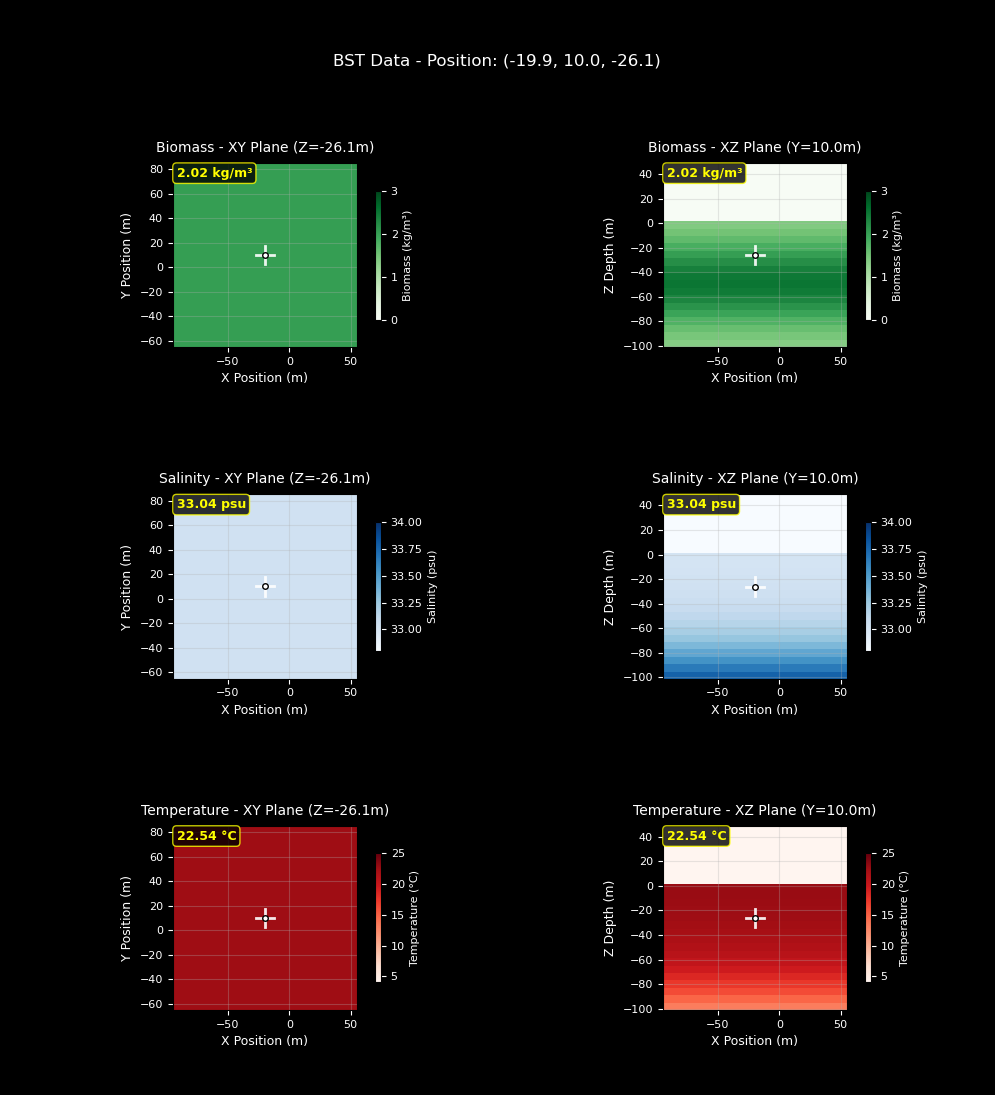
Default Configuration:
scenario = {
"name": "test_currents",
"world": "PierHarbor",
"package_name": "Ocean",
"main_agent": "auv0",
"ticks_per_sec": 60,
"frames_per_sec": 60,
"agents": [
        {
            "agent_name": "auv0",
            "agent_type": "HoveringAUV",
            "sensors": [
                {
                    "sensor_type": "BSTSensor",
                    "socket": "COM",
                    "configuration":{}
                },
                {
                    "sensor_type": "LocationSensor",
                    "socket": "COM"
                }
            ],
        "control_scheme": 0,
        "location": [-20, 10, -10]
        }
    ],
}
Customized Configuration
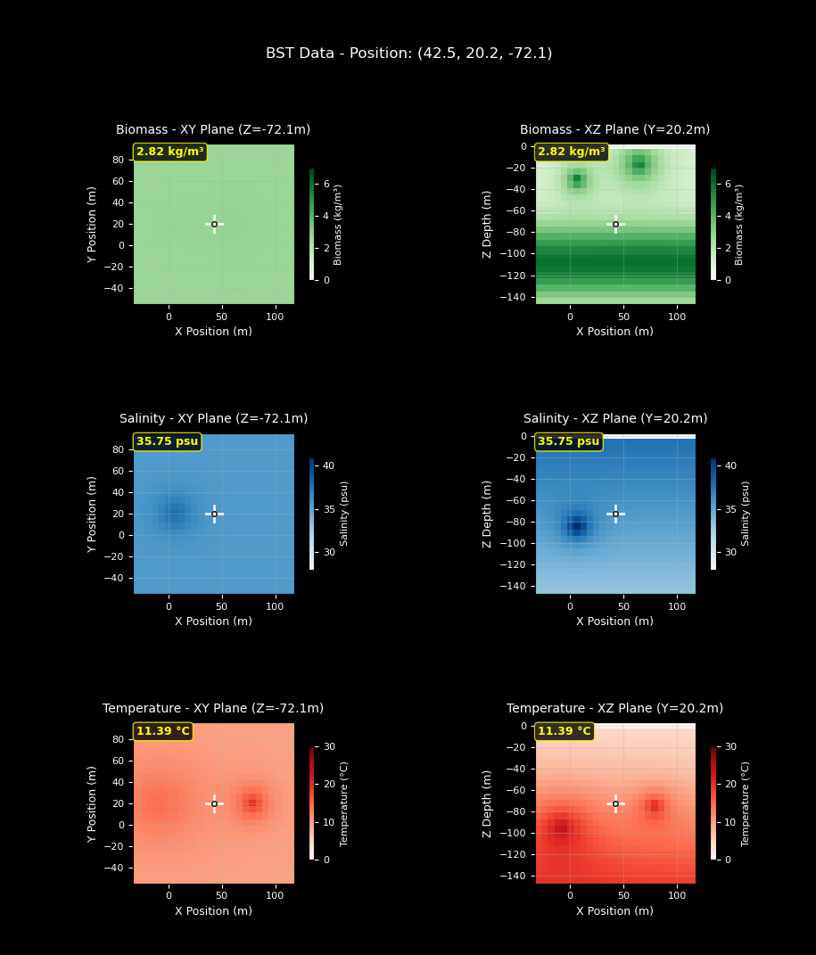
Customized Configuration Parameters:
{
    "sensor_type": "BSTSensor",
    "socket": "COM",
    "Hz": 1,
    "configuration": {
        "max_biomass": 6,
        "biomass_range": (0, 7),
        "peak_depth": 110.0,
        "biomass_clusters": [
            {
                "position": [65, 20, -15],
                "strength": 5,
                "falloff": 15
            },
            {
                "position": [5, 20, -30],
                "strength": 5,
                "falloff": 10
            }
        ],
        "surface_psu": 40,
        "deep_psu": 30,
        "halocline_depth": 90,
        "halocline_thickness": 75,
        "salinity_range": (28, 41),
        "salinity_clusters": [
            {
                "position": [5, 20, -85],
                "strength": 8,
                "falloff": 10
            }
        ],
        "surface_temp": 2,
        "deep_temp": 26,
        "thermocline_depth": 110,
        "thermocline_thickness": 50,
        "temperature_range": (0, 30),
        "temperature_clusters": [
            {
                "position": [80, 20, -75],
                "strength": 12,
                "falloff": 12
            },
            {
                "position": [-10, 20, -95],
                "strength": 12,
                "falloff": 25
            }
        ]
    }
}
Custom Functions
Because implementing custom functions involves more than just changing config parameters, we’ve only included the
custom functions that were passed into our HoloOceanEnvironment.initialize_bst_graphs function call. If you’d
like to see the full implementation for custom functions, see the Sampling Biomass, Salinity, Temperature example.
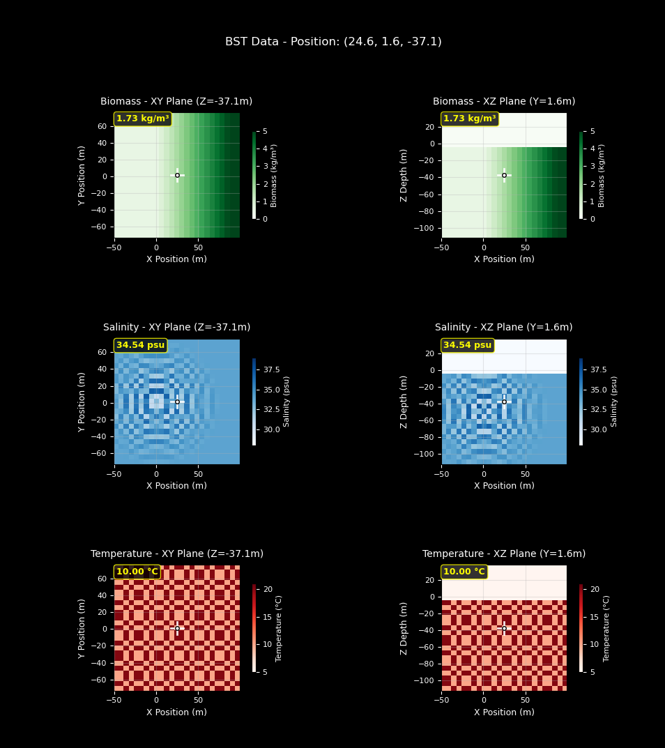
Custom Functions and Configuration Parameters:
def biomass_fx(location):
    # NOTE: It's required that we name this parameter "location"
    x, y, z = location
    x_fade = max(0, min(1, x / 100))  # fades from 0 at x=0.5 to 5.5 at x=100, then stays at 5.5
    return 5.0 * x_fade + 0.5

def salinity_fx(location):
    # This function creates decaying oscillations that originate from a single point
    import math
    x, y, z = location
    center = [0, 0, -50]
    # The zip() function in Python pairs corresponding values in two iterables together in tuples
    dist = math.sqrt(sum((a - b)**2 for a, b in zip(location, center)))
    if dist > 80:
        return 34  # base salinity
    amplitude = 4 * (1 - dist/80)
    return 34 + amplitude * math.cos(dist * 2 * math.pi / 10)

def temperature_fx(location):
    # This function creates a checkerboard-type pattern across the world
    x, y, z = location
    square_size = 5
    checks = sum(int(coord // square_size) % 2 for coord in [x, y, z])
    return 10 if checks % 2 == 0 else 20  # alternate between two temps

scenario = {
    "name": "BST Custom Functions",
    "main_agent": "auv0",
    "ticks_per_sec": 60,
    "frames_per_sec": 60,
    "agents": [
            {
                "agent_name": "auv0",
                "agent_type": "HoveringAUV",
                "sensors": [
                    {
                        "sensor_type": "BSTSensor",
                        "socket": "COM",
                        "configuration": {
                            "biomass_range": (0, 5),
                            "salinity_range": (28, 39),
                            "temperature_range": (5, 21)
                        }
                    },
                    {
                        "sensor_type": "LocationSensor",
                        "socket": "COM"
                    }
                ],
            "control_scheme": 0,
            "location": [-20, 10, -10]
            }
        ],
    }